Part I: Introduction
For many years, Value at Risk has been widely utilized by financial institutions to estimate the risk level for an investment. More specially, it's a statistical technique used to measure the amount of loss that could happen over a certain period.
This single number can give us a rough idea about the risk level for any assets we are interested in, which is easy to understand and interpret. Because of that, deriving a reasonable and accurate VaR can help investors manage their investment strategy effectively.
Hull and White(1998) suggest incorporating volatility into estimating VaR.
Volatility is defined as the standard deviation of the stock's daily return. Although volatility is not the same as risk, changes in stock volatility have been a significant concern for investors because of the acknowledged connection between volatility and risk,
according to Koima, Mwita, and Nassiuma (2015). For that reason, having an accurate estimation of volatility can help us derive a more reasonable VaR.
In this project, we first tested the traditional volatility estimation approach on a Chinese stock index, specifically CSI 300.
Then, we incorporated several machine learning algorithms to make the same estimation because we are curious about whether modern machine learning techniques can help in the financial risk assessment. Finally, we backtested our estimation on the real historical data,
and calculated the violation ratio for each underestimation to compare our model accuracy.
Part II: Brief Literature Review
Over the past decades, many techniques have been introduced to modeling volatility in the stock market, including MA, EWMA, and GARCH models. However, there does not seem to be a consensus about which model is better in predicting accuracy.
Lee and Nguyen (2017) suggested that the GARCH(1,1) model was the most robust one in their study of predicting volatility in the emerging markets. While, according to Galdi and Pereira (2007), VaR calculated using MA and EWMA models suffer fewer violations than that of the GARCH model.
As a result, in this project, we decided to test the performance of all three conventional models and compare their forecasting accuracy.
In addition to modeling volatility using the conventional methods, in recent years, applying Machine Learning algorithms in financial risk assessment has become a popular and rising topic in both academia and industry.
Mittnik, Robinzonov, and Spindler (2015) applied boosting techniques to derive monthly volatility predictions for S&P 500 and suggested that their approach substantially improves out-of-sample volatility forecasts for short- and longer-run horizons compared with conventional GARCH and EGARCH models.
In their study of predicting realized variance for DJIA, Christensen, Siggaard, and Veliyev(2021) have proven that Random Forest and Neural Network can significantly improve the predicting accuracy compared with the HAR model when adding other predictors in the dataset.
In this project, because we don't have access to the intraday data, we calculated the quantiles of the distribution for the 20-day log return to represent the daily loss as our dependent variable, suggested by Ying L. Becker ET AL.(2020) in their research, and built four machine learning models to predict the daily loss directly.
And compare this result with that estimated through modeling volatility using the conventional method. Specifically, with the help of some other predictors, we would like to see whether machine learning models outperform the traditional model in estimating VaR.
Part III: Data and Methodology
3.1 Data Description
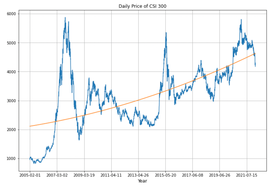
We downloaded CSI 300 ticker data from 2005-02-01 to 2022-03-14 on Investing.com ranging as our primary dataset. The CSI 300 is a capitalization-weighted stock market index designed to replicate the performance of the top 300 stocks traded on the Shanghai Stock Exchange and the Shenzhen Stock Exchange.
The original dataset contains 4160 observations.
When we are making predictions using machine learning algorithms, in addition to use the features engineered from the primary dataset, including the Return Variance, Daily Spread, Month of the Year, we also expanded our dataset by adding another nine assets as predictors,
including two additional stock indexes, five commodities, China's 10-year Bond Yield Rate, and the Chinese Yuan to US dollar exchange rate. To keep the data consistent, we mapped all the data on the date index of CSI 300 and filled the missing data using the average of two closest valid values,
one from the preceding day and another from the following day.
What's more, because we don't have access to the intraday stock index data required to estimate the realized volatility,
we decided to use the quantiles of the distribution of log return, which represents the potential daily loss directly, as our dependent variable.
And we want our results using the machine learning models to be comparable with that using the conventional methods. We think a similar rolling window approach should be appropriate in finding the quantile values.
So, for every twenty days, we estimate the 2.5% quantiles of the daily log return for CSI 300 and all other features we selected for our research. (We logged all values to ensure the numbers are within the same scale)
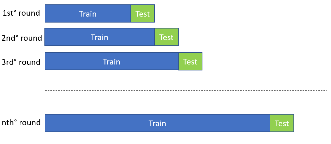
Finally, we constructed training and testing sample based on the time horizon to ensure our model validity. The training set contains 3640 data from 2005-02-01 to 2020-01-16, while the testing set contains 520 data from 2020-01-17 to 2022-03-14.
Data Preview Download Full Dataset
>View Code Details for Data Preprocess
3.2 Modelling Methodology
3.2.1 Conventional Models
We first estimaed the daily volatility of the 20-day rolling window using MA and EWMA method based on the following formula.
$$ MA: {\sigma_{t}^2 = \frac{1}{m} \sum_{j=0}^{m-1} R_{t-j}^2 }\quad[1]$$ $$ EWMA: {\sigma_{t}^2 = (1-\lambda)(R_{t-1}^2 + \lambda R_{t-2}^2 + \lambda^2 R_{t-3}^2 + ... + \lambda^{m-1} R_{t-m}^2) + \lambda^m \sigma_{t-m}^2 }\quad[2]$$
Then, we choose the GARCH(1,1) model to predict daily volatility and used the maximum likelihood estimation to find optimal parameters in the GARCH model. where v is the return variance, and ui is the daily return $$ \textit{Maximum Likelihood Estimation: } {LL = \sum_{i=1}^{m}[-ln(v) - \frac{u_{i}^2}{v}] } \quad[3]$$
$$ GARCH(1,1): {\sigma_{t}^2 = \alpha_0 + \alpha_1(R_{t}-\mu)^2 + \beta \sigma_{t-1}^2 } \quad[4]$$
After we get an estimate of the volatility(σt), we used the following formula to find the 2.5% VaR for each model, where µ is the mean of return in the training sample, and Rcrit is the critical value at the 2.5% of the standardized historical distribution of log return in the training sample. $$R_{t}^* = \mu + R_{crit} \sigma_t \quad[5]$$
3.2.2 Machine Learning Models
Selected Models: Regression with ridge/lasso regularization, Random Forest, Gradient Boosting, and Recurrent Neural Network.
Prediction Period: We designed our model to make multiple days ahead one-time forecasts. Specifically, making predictions for the next twenty day at once.
During training, we divided our data on a monthly basis (each month contains twenty days) and used walking forward validation method to train the models.In this way,
our model gradually makes predictions and validates on the following month; after each iteration, it will combine the validating set and the previous training set to construct another training set for the next step.
We also applied grid search for the first four algorithms to find the optimal hyperparameters.
About Neural Network:
To match the input shape for the multi-step forecast we designed, specially making predictions for the consecutive twenty days at one time,
and to ensure there are enough data to train the neural network, we used this rolling technique and reconstructed our training dataset for the neural network.
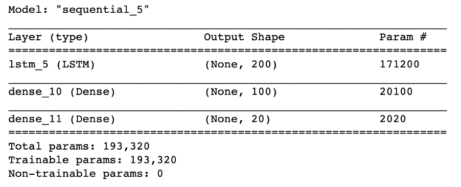
Concerning the network architecture, Hamida and Iqbalb(2004) suggested that one hidden layer may be sufficient to map the input to output for most financial data.
We manually did several casual searches for the neural in each layer and selected the best one among these searches. The final structure of our neural network is shown below.
For both layers, we used sigmoid activation function, MSE as the loss function, and Adam optimizer as the model optimizer. Finally, We added early stopping in the training stage to avoid overfitting.
Finally, we tested the model performance on the testing sample: again using walking forward method to make predictions for each month and used the following two measures to estimate the predictive accuracy, where n is the total number of days in one predictions, and T is the number of predictions. $${ R_{m}^2 = 1 - \frac{\sum_{i=1}^{n}(y_i - \hat y_i)^2}{\sum_{i=1}^{n}(y_i - \bar y)^2} } \quad { R^2 = \frac{1}{T} \sum_{m=1}^{T} R_{m}^2 } \quad[6]$$ $${RMSE_m = \sqrt {\frac{1}{n}\sum_{i=1}^{n}(y_i - \hat y_i)^2}} \quad {RMSE = \frac{1}{T} \sum_{m=1}^{T} RMSE_m} \quad[7]$$ The sample code shown below is the function we defined to calculate the two measurements.
					# SAMPLE CODE #
def predAccuracy(X,y,X_test,y_test,best_model):
	X_new = X.copy()
	y_new = y.copy()
	R2  = []
	RMSE = []
	Y_pred = []
	i = 0
	while i < len(test):
		start = i
		end   = i+20
		X_test_new = X_test[start:end].copy()
		y_test_new = y_test[start:end].copy()
		best_model.fit(X_new,y_new)
		y_pred = best_model.predict(X_test_new)
		rmse = np.sqrt(mean_squared_error(y_test_new,y_pred))
		r2  = best_model.score(X_test_new,y_test_new)
		R2.append(r2)
		RMSE.append(rmse)
		Y_pred += list(y_pred)

		X_new = np.concatenate((X_new, X_test[start:end]), axis=0)
		y_new += y_test_new
		i +=20
	return R2,RMSE,Y_pred
Part IV: Model Estimation and Analysis
Our objective is to estimate the 20-day 2.5% VaR for this stock index, an alternative way to interpret this measure is we are 97.5% confident
that after 20 days holding this stock, our loss will not greater than VaR. As a result, one metric can be used to measure the predicted VaR is
compare the expected value with the actual return, and count the times that the actual return is smaller than the predicted value, which is called VaR exceptions,
and calculate the relative percentage of exceptions(Violation Ratio) for the whole predictive period.
If VR is close to one, it means that about 2.5% of the time our loss is greater than VaR, namely our model capture the risk level just as we would expect.
Violation Ratio is calculated using formula 8, where v is the number of exceptions, p is the expected ratio of exceptions, and WT is the lenth of the period under study.
$$VR = \frac{v}{pW_t} \quad[8]$$
4.1 Conventional Models
First, we calculated exceptions and VR of three different models based on the out of sample dataset, as shown in Table 1. The result indicates that given the two year testing period, MA is best model to use, it's violation ratio is closest to 1 while EWMA tends to underestimate risk more and while the GARCH model tends to overestimate risk.
| Models | Exceptions | VR |
| MA | 0.0288 | 1.15 |
| EWMA | 0.0403 | 1.61 |
| GARCH(1,1) | 0.0076 | 0.31 |
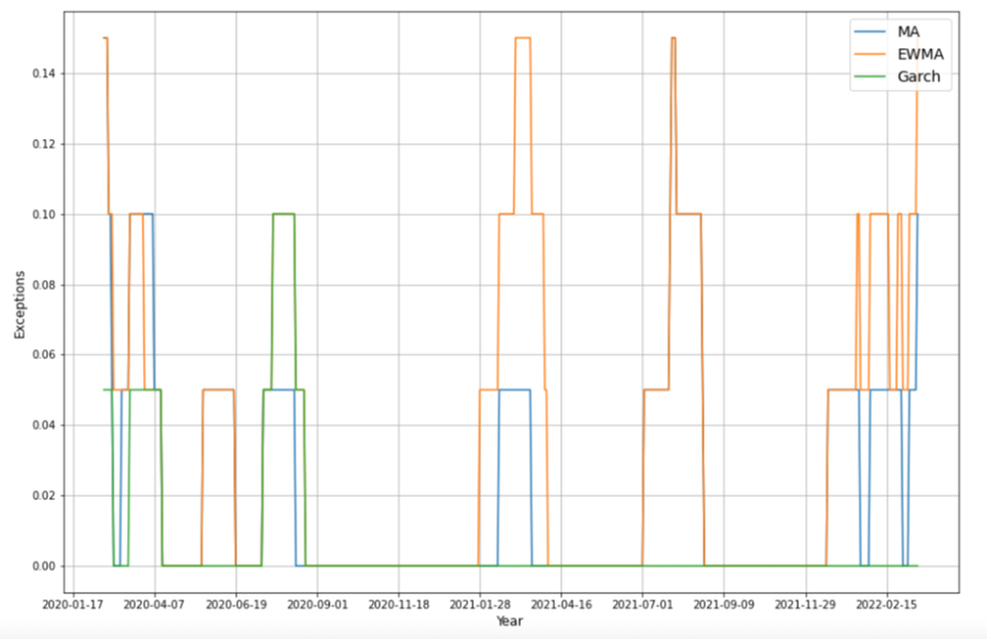
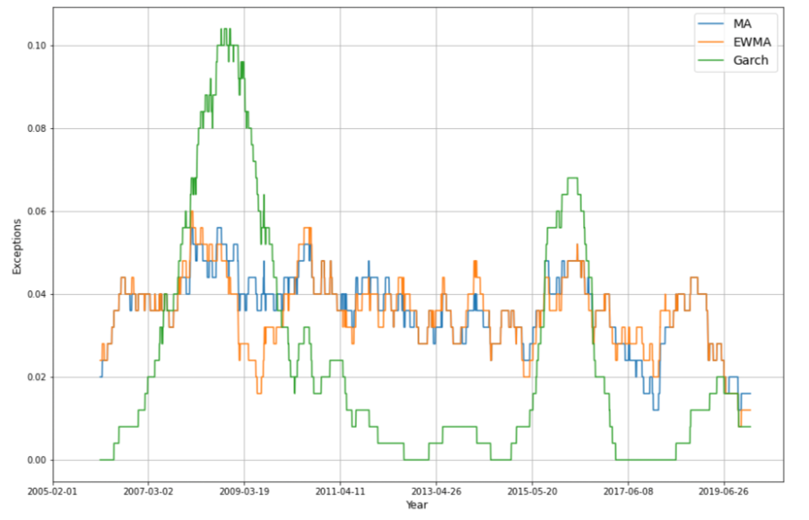
To get more intuitive information, we plot the change rate of exceptions over various rolling windows on the out-of-sample data. The plot below shows one of the visualizations with the window size of 20.
It is quiet obvious that the MA is the best among three methods, on average it's exceptions is aboue 2.5% with the smallest fluctations compared with the rest two models.
However, this result seems counterintuitive to us, especially the comparison between MA and EWMA models. Therefore, we conducted the same analysis on the in-sample data, which contains a longer period.
From the results demonstrated below, we noticed that for the in-sample data, GARCH(1,1) model has the smllest violation ratio among the three, while the estimation using MA and EWMA becomes closer, both underestimate risk to a similar extent.
If we looked at the exception plot, it is clear that even though this time the VR of the GARCH(1,1) model is the closet to one, the predictions using GARCH mdoel is also the most volatile. It can produce better forecasts for some periods, while the errors could be too big to be accepted in others.
In the case of modeling volatility, if we don't have additional information suggesting which period we are at when making predictions, we would love to have predictions to be within a relatively constant range; this oscillation makes the GARCH model less preferable.
Regarding the results of MA and EWMA model, we think a more extended testing period will help us examine the true performance of our model, while it's worth noting that here we used in-sample data to inspect the long-term performance checking, which has a potential problem of data leakage.
With all being considered, we think in the current study, the out of sample test result is more credible.
Overall, the best model we would recommend within the conventional methods is the Moving Average Model with the testing violation ratio of 1.15.
| Models | Exceptions | VR |
| MA | 0.0346 | 1.38 |
| EWMA | 0.0340 | 1.36 |
| GARCH(1,1) | 0.0228 | 0.91 |
4.2 Machine Learning Algorithms
First, we compared model forecasting accuracy using the two metrics we chose. Table 3 shows the summary of each model with the optimal parameters we chose and the corresponding estimation measurement. We noticed a discrepancy between the two measures used to estimate the model accuracy from the results. All the R-squared calculated for the twenty-day rolling predictions are negative. On the contrary, the mean squared error indicates that our models have made a robust prediction. To figure out the reason behind this phenomenon, we tried to make predictions for all the testing samples at once. The results are also listed in the table below, with a more extended forecasting period, R-squared has improved a lot, and the mean squared error did not change significantly.
| 20-day rolling forecast | 2-year one-time forecast | ||||
| Models | Hyperparameters | Testing R2 | Testing RMSE | Testing R2 | Testing RMSE |
| Ridge Regression | α = 0.5 | -5.500 | 0.0031 | 0.8689 | 0.0042 |
| Lasso Regression | α = 0.000055 | -3.910 | 0.0030 | 0.8856 | 0.0039 |
| Random Forest | Max_depth=10, Max_features=10 |
-7.274 | 0.0029 | 0.9939 | 0.0039 |
| Gradient Boosting | Max_depth=3, Max_features=13 |
-6.882 | 0.0031 | 0.9417 | 0.0009 |
| Recurrent Neural Networks | -2.801 | 0.0135 | |||
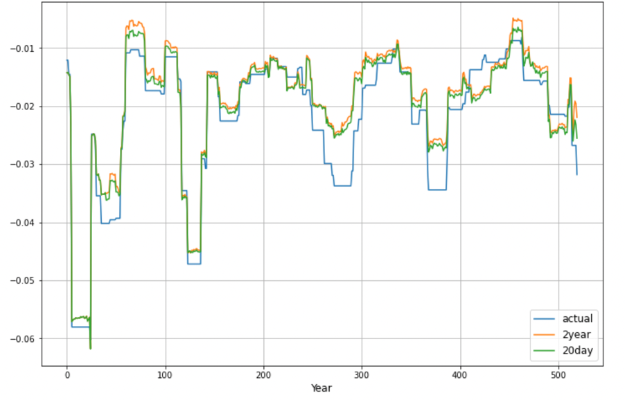
Due to the inconsistency in the two measurements, we suspect that the forecasting period might affect our prediction accuracy, so we plotted the two sets of predictions for each of the models and compared that with our actual target variable. The figure below shows the one of ridge regression; As indicated by the line chart, forecasts of the two settings are almost identical, which is in line with the mean squared error estimator. Thus, we conclude that in this case, mean squared error should be a better indicator for measuring our model accuracy. As such, all of our four models can give accurate predictions with only minor errors.
Again, what we really concerned about is how accurate the VaR derived from our forecasting models, we compared the predicted loss with the actual loss using backtesting and calculated the violation ratio to test the model accuracy. As shown in Table 4, VaR estimated using Recurrent Neural Network is the most accurate, since its violation ratio is most close to one, given the 2.5% confidence level we defined. All the other four models underestimate the stock risk level.
| Models | Exceptions | VR |
| Ridge Regression | 0.0788 | 3.15 |
| Lasso Regression | 0.0769 | 3.07 |
| Random Forest | 0.0788 | 3.15 |
| Gradient Boosting | 0.0731 | 2.92 |
| RNN | 0.0230 | 0.92 |
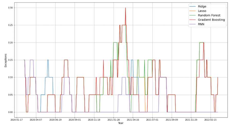
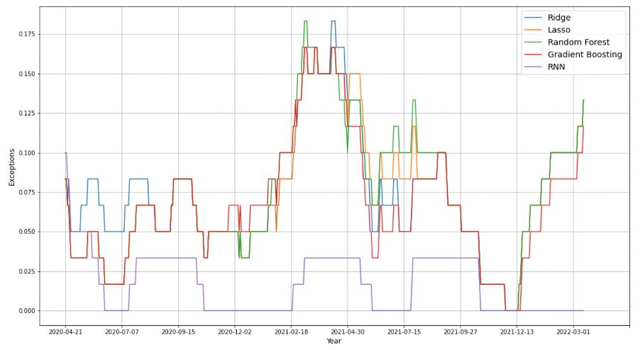
To visualize the change in the percentage of exceptions over the testing period, we made the following three plots of exceptions rate using different settings of the rolling window size. As the observation period extends, the difference between RNN and the other models becomes much clearer, it can always generate a 2.5% VaR at 2.5%. We presume that compared with other machine learning algorithms, RNN with the LSTM cells can remember the important characteristics about the input, which allows it to guess what might happen in the next period.
Part V: Conclusion And Future Study
GARCH, MA, and EWMA remain very crucial risk prediction methods. All of them have some strengths and weaknesses. This research compared the Root of Mean Squared Error, exceptions, and violation ratio of daily loss among three conventional methods and five machine learning methods to find out the best model to predict the CSI 300 stock.
For conventional methods, we prefer to use MA model; but we'd like to mention that in the future study, leave out a clean testing sample contains a much longer period might produce a more robust result and help us understanding the model performace better.
RNN performs the best within all machine learning methods in exceptions(0.023) and VR(0.92). Our final conclusion is that RNN can improve forecasting accuracy compared with conventional methods, which improved the predicting accuracy by 7%. Besides, machine learning methods can achieve multiple-day ahead forecasts compared with conventional methods that can only make one-day ahead predictions.
Nevertheless, in our research, we have introduced several features in the RNN to help us make predictions. In reality, doing so will notably increase the computing time and the difficulties of data management. So, before using the machine learning models to make predictions, we think it will be helpful to perform some formal feature engineering and select the most relevant ones that should add to the model.
In addition, when we are using maximum likelihood estimating the parameters for GARCH(1,1) model, we have run into some converging issues, we still need to do further research on this subject and see if we can improve the GARCH model estimations. And same problem with tuning hyperparameters for RNN, as we learn more about the recurrent neural network in the future, we might be able to select the hyperparameters more intellectually.